Post-processing
In this section, we discuss how to access and work with data from optimization records. This includes loading various data, visualizing results, and hot-starting an optimization using optimization records.
Recording an optimization
We start by recording an optimization, as discussed in the previous section.
The problem is the same as before, and we use the TrustConstr optimizer.
import numpy as np
import modopt as mo

x0 = np.array([50., 5.])            # initial guess
xl = np.array([0., -np.inf])        # variable lower bounds
cl = np.array([1., 1.])             # constraint lower bounds
cu = np.array([1., np.inf])         # constraint upper bounds
c_scaler = np.array([10., 100.])    # constraint scaler

def obj(x):
    return np.sum(x**2)
def grad(x):
    return 2 * x
def con(x):
    return np.array([x[0] + x[1], x[0] - x[1]])
def jac(x):
    return np.array([[1., 1], [1., -1]])

# Define the problem as a ProblemLite object
# A ProblemLite object acts as a container for the problem constants, functions, and their derivatives
problem = mo.ProblemLite(
    x0,
    obj=obj,
    grad=grad,
    con=con,
    jac=jac,
    cl=cl,
    cu=cu,
    xl=xl,
    c_scaler = c_scaler,
    name='constrained_quadratic'
    )

optimizer = mo.TrustConstr(problem=problem,
                           solver_options={'maxiter': 100, 'gtol': 1e-12},
                           recording=True)
results   = optimizer.solve()
optimizer.print_results()

# Print the directory and its contents to see the generated output files
print('Output Directory:', optimizer.out_dir)
print('Output Files:', optimizer.modopt_output_files)
	Solution from Scipy trust-constr:
	----------------------------------------------------------------------------------------------------
	Problem                       : constrained_quadratic
	Solver                        : scipy-trust-constr
	Method                        : tr_interior_point
	Success                       : True
	Message                       : `gtol` termination condition is satisfied.
	Status                        : 1
	Total time                    : 0.14261221885681152
	Objective                     : 1.0000320268995626
	Gradient norm                 : 2.000032026643136
	Optimality                    : 4.3125588820511207e-13
	Max. constr. violation        : 0.0
	Trust region radius           : 639535.7360242795
	Constraint penalty            : 1.0
	Barrier parameter             : 3.200000000000001e-05
	Barrier tolerance             : 3.200000000000001e-05
	Total function evals          : 13
	Total gradient evals          : 13
	Total Hessian evals           : 0
	Total constraint evals        : 13
	Total constr. Jacobian evals  : 13
	Total constr. Hessian evals   : 0
	Total iterations              : 18
	CG iterations                 : 12
	CG stop condition             : 1
	Total callbacks               : 52
	Reused callbacks              : 0
	obj callbacks                 : 13
	grad callbacks                : 13
	hess callbacks                : 0
	con callbacks                 : 13
	jac callbacks                 : 13
	----------------------------------------------------------------------------------------------------
Output Directory: constrained_quadratic_outputs/2025-02-03_12.25.55.893290
Output Files: ['directory: constrained_quadratic_outputs/2025-02-03_12.25.55.893290', 'modopt_results.out', 'modopt_summary.out', 'record.hdf5']
Viewing record contents
To view the data available in a record, call the print_record_contents() utility with the record file name,
as shown below.
There are four types of information available in a record: attributes, opt_vars, callback_vars, and results.
The print_record_contents() function always returns a tuple containing four lists, one for each type of information.
To suppress printing, set the keyword argument suppress_print=True.
from modopt.postprocessing import print_record_contents
record_contents = print_record_contents(optimizer.out_dir+'/record.hdf5')
Available data in the record:
-----------------------------
 - Attributes of optimization    : ['c_lower', 'c_scaler', 'c_upper', 'constrained', 'hot_start_from', 'modopt_output_files', 'nc', 'nx', 'o_scaler', 'problem_name', 'readable_outputs', 'recording', 'solver_name', 'solver_options-barrier_tol', 'solver_options-callback', 'solver_options-factorization_method', 'solver_options-gtol', 'solver_options-ignore_exact_hessian', 'solver_options-initial_barrier_parameter', 'solver_options-initial_barrier_tolerance', 'solver_options-initial_constr_penalty', 'solver_options-initial_tr_radius', 'solver_options-maxiter', 'solver_options-sparse_jacobian', 'solver_options-verbose', 'solver_options-xtol', 'timestamp', 'visualize', 'x0', 'x_lower', 'x_scaler', 'x_upper']
 - Recorded optimizer variables  : ['barrier_parameter', 'barrier_tolerance', 'cg_niter', 'cg_stop_cond', 'con', 'constr_penalty', 'feas', 'grad', 'iter', 'jac', 'lgrad', 'lmult_c', 'lmult_x', 'ncev', 'ncgev', 'nchev', 'nfev', 'nfgev', 'nfhev', 'obj', 'opt', 'time', 'tr_radius', 'x']
 - Recorded callback variables   : ['con', 'grad', 'jac', 'obj', 'x']
 - Results of optimization       : ['barrier_parameter', 'barrier_tolerance', 'cg_niter', 'cg_stop_cond', 'con', 'con_evals', 'constr_penalty', 'feas', 'grad', 'grad_evals', 'hess_evals', 'iter', 'jac', 'jac_evals', 'lgrad', 'lmult_c', 'lmult_x', 'message', 'method', 'ncev', 'ncgev', 'nchev', 'nfev', 'nfgev', 'nfhev', 'obj', 'obj_evals', 'opt', 'out_dir', 'reused_callbacks', 'status', 'success', 'time', 'total_callbacks', 'tr_radius', 'x']
Loading results and attributes
Attributes and results of an optimization can be loaded as dictionaries
by calling the load_attributes() and load_results() utility functions
with the record file name, as shown below.
from modopt.postprocessing import load_attributes, load_results
attributes = load_attributes(optimizer.out_dir+'/record.hdf5')
results    = load_results(optimizer.out_dir+'/record.hdf5')

print("Attributes:")
print(attributes)

print("Results:")
print(results)
Attributes:
{'c_lower': array([1., 1.]), 'c_scaler': array([ 10., 100.]), 'c_upper': array([ 1., inf]), 'constrained': True, 'hot_start_from': 'None', 'modopt_output_files': ['directory: constrained_quadratic_outputs/2025-02-03_12.25.55.893290', 'modopt_results.out', 'modopt_summary.out', 'record.hdf5'], 'nc': 2, 'nx': 2, 'o_scaler': array([1.]), 'problem_name': 'constrained_quadratic', 'readable_outputs': [], 'recording': 'True', 'solver_name': 'scipy-trust-constr', 'solver_options-barrier_tol': 1e-08, 'solver_options-callback': 'None', 'solver_options-factorization_method': 'None', 'solver_options-gtol': 1e-12, 'solver_options-ignore_exact_hessian': False, 'solver_options-initial_barrier_parameter': 0.1, 'solver_options-initial_barrier_tolerance': 0.1, 'solver_options-initial_constr_penalty': 1.0, 'solver_options-initial_tr_radius': 1.0, 'solver_options-maxiter': 100, 'solver_options-sparse_jacobian': 'None', 'solver_options-verbose': 0, 'solver_options-xtol': 1e-08, 'timestamp': '2025-02-03_12.25.55.893290', 'visualize': [], 'x0': array([50.,  5.]), 'x_lower': array([  0., -inf]), 'x_scaler': array([1., 1.]), 'x_upper': array([inf, inf])}
Results:
{'barrier_parameter': 3.200000000000001e-05, 'barrier_tolerance': 3.200000000000001e-05, 'cg_niter': 12, 'cg_stop_cond': 1, 'con': array([ 10.        , 100.00320264]), 'con_evals': 13, 'constr_penalty': 1.0, 'feas': 0.0, 'grad': array([ 2.00003203e+00, -3.20263867e-05]), 'grad_evals': 13, 'hess_evals': 0, 'iter': 18, 'jac': array([[  10.,   10.],
       [ 100., -100.]]), 'jac_evals': 13, 'lgrad': array([ 4.31139106e-13, -4.31255888e-13]), 'lmult_c': array([-0.0999984 , -0.01000016]), 'lmult_x': array([-3.1999488e-05,  0.0000000e+00]), 'message': '`gtol` termination condition is satisfied.', 'method': b'tr_interior_point', 'ncev': 13, 'ncgev': 13, 'nchev': 0, 'nfev': 13, 'nfgev': 13, 'nfhev': 0, 'obj': 1.0000320268995626, 'obj_evals': 13, 'opt': 4.3125588820511207e-13, 'out_dir': 'constrained_quadratic_outputs/2025-02-03_12.25.55.893290', 'reused_callbacks': 0, 'status': 1, 'success': True, 'time': 0.13321709632873535, 'total_callbacks': 52, 'tr_radius': 639535.7360242795, 'x': array([ 1.00001601e+00, -1.60131934e-05])}
Loading variable iterates
The load_variables() utility function loads variable iterates from the record.
This function requires two arguments: 1) the record file name, and 2) the list of variable names to load.
The function returns a dictionary with keys as variable names and values as lists of variable iterates
corresponding to those variable names.
Note that the keys for callback_variables will be prefixed with 'callback_'.
If only specific scalar variables need to be loaded from an array variable, use the format 'var_name[idx]'.
For example,
'x[0]'will load the iterates for the first element of the array ‘x’, and'jac[i,j]'will load the iterates for the (i,j)-th element of the array ‘jac’.
The load_variables() function also provides an optional keyword argument, callback_context,
to load callback_variables together with its corresponding inputs.
To learn more about callback_context, visit the API Reference.
The following code loads the iterates of x[0], the objective, the Jacobian, optimality, and feasibility from the record.
from modopt.postprocessing import load_variables
vars = load_variables(optimizer.out_dir+'/record.hdf5', ['x[0]', 'obj', 'jac', 'opt', 'feas'])

print('Loaded variables:')
print(vars.keys())

# Print the loaded variable iterates
for key, value in vars.items():
    print('\n', key, ':')
    print(value)
Loaded variables:
dict_keys(['x[0]', 'callback_x[0]', 'obj', 'callback_obj', 'jac', 'callback_jac', 'opt', 'feas'])

 x[0] :
[50.0, 49.06680741392834, 42.1402716614226, 13.137131926669479, 3.265462548872426, 1.426337395295874, 1.1484153222707345, 1.0661629237127606, 1.0661629237127606, 1.0170864850904997, 1.0170864850904997, 1.0026442417982402, 1.0026442417982402, 1.0004156095347128, 1.0004156095347128, 1.0000803575038417, 1.0000803575038417, 1.0000160131933589]

 callback_x[0] :
[50.0, 50.0, 50.0, 50.0, 49.06680741392834, 49.06680741392834, 49.06680741392834, 49.06680741392834, 42.1402716614226, 42.1402716614226, 42.1402716614226, 42.1402716614226, 13.137131926669479, 13.137131926669479, 13.137131926669479, 13.137131926669479, 3.265462548872426, 3.265462548872426, 3.265462548872426, 3.265462548872426, 1.426337395295874, 1.426337395295874, 1.426337395295874, 1.426337395295874, 1.1484153222707345, 1.1484153222707345, 1.1484153222707345, 1.1484153222707345, 1.0661629237127606, 1.0661629237127606, 1.0661629237127606, 1.0661629237127606, 1.0170864850904997, 1.0170864850904997, 1.0170864850904997, 1.0170864850904997, 1.0026442417982402, 1.0026442417982402, 1.0026442417982402, 1.0026442417982402, 1.0004156095347128, 1.0004156095347128, 1.0004156095347128, 1.0004156095347128, 1.0000803575038417, 1.0000803575038417, 1.0000803575038417, 1.0000803575038417, 1.0000160131933589, 1.0000160131933589, 1.0000160131933589, 1.0000160131933589]

 obj :
[2525.0, 2431.6089501192855, 1791.1150473325854, 172.71635837369885, 11.873365835978536, 2.216201939847089, 1.3408848603109211, 1.1410809123739623, 1.1410809123739623, 1.0347568661264952, 1.0347568661264952, 1.0053024676258553, 1.0053024676258553, 1.000831564531996, 1.000831564531996, 1.0001607279223403, 1.0001607279223403, 1.0000320268995626]

 callback_obj :
[2525.0, 2431.6089501192855, 1791.1150473325854, 172.71635837369885, 11.873365835978536, 2.216201939847089, 1.3408848603109211, 1.1410809123739623, 1.0347568661264952, 1.0053024676258553, 1.000831564531996, 1.0001607279223403, 1.0000320268995626]

 jac :
[array([[  10.,   10.],
       [ 100., -100.]]), array([[  10.,   10.],
       [ 100., -100.]]), array([[  10.,   10.],
       [ 100., -100.]]), array([[  10.,   10.],
       [ 100., -100.]]), array([[  10.,   10.],
       [ 100., -100.]]), array([[  10.,   10.],
       [ 100., -100.]]), array([[  10.,   10.],
       [ 100., -100.]]), array([[  10.,   10.],
       [ 100., -100.]]), array([[  10.,   10.],
       [ 100., -100.]]), array([[  10.,   10.],
       [ 100., -100.]]), array([[  10.,   10.],
       [ 100., -100.]]), array([[  10.,   10.],
       [ 100., -100.]]), array([[  10.,   10.],
       [ 100., -100.]]), array([[  10.,   10.],
       [ 100., -100.]]), array([[  10.,   10.],
       [ 100., -100.]]), array([[  10.,   10.],
       [ 100., -100.]]), array([[  10.,   10.],
       [ 100., -100.]]), array([[  10.,   10.],
       [ 100., -100.]])]

 callback_jac :
[array([[  10.,   10.],
       [ 100., -100.]]), array([[  10.,   10.],
       [ 100., -100.]]), array([[  10.,   10.],
       [ 100., -100.]]), array([[  10.,   10.],
       [ 100., -100.]]), array([[  10.,   10.],
       [ 100., -100.]]), array([[  10.,   10.],
       [ 100., -100.]]), array([[  10.,   10.],
       [ 100., -100.]]), array([[  10.,   10.],
       [ 100., -100.]]), array([[  10.,   10.],
       [ 100., -100.]]), array([[  10.,   10.],
       [ 100., -100.]]), array([[  10.,   10.],
       [ 100., -100.]]), array([[  10.,   10.],
       [ 100., -100.]]), array([[  10.,   10.],
       [ 100., -100.]])]

 opt :
[44.97317172737661, 44.10755536872242, 38.16378116721319, 12.56369482254608, 3.616883389849403, 0.4254477324883117, 0.03805897490957255, 0.002850769190926694, 0.008402289887398908, 0.0002561569722679402, 0.000533892876432962, 3.453049888618026e-06, 1.1936761440439064e-05, 1.3123963654433461e-08, 2.7922443006974523e-07, 5.84988753130674e-11, 1.0345085697445759e-08, 4.3125588820511207e-13]

 feas :
[540.0, 529.716377192246, 450.53397219603494, 125.0061936108822, 11.654079239150402, 1.7763568394002505e-15, 1.7763568394002505e-15, 1.7763568394002505e-15, 1.7763568394002505e-15, 1.7763568394002505e-15, 1.7763568394002505e-15, 0.0, 0.0, 0.0, 0.0, 0.0, 0.0, 0.0]
Visualizing recorded optimization
A recorded optimization can be visualized using the visualize() function from the post-processing utilities.
This function plots scalar variables after loading them from the record.
The two required arguments are: 1) the record file name, and 2) the list of variable names to visualize.
The final optimization plot can be saved to a file by setting the keyword argument save_figname,
which is None by default.
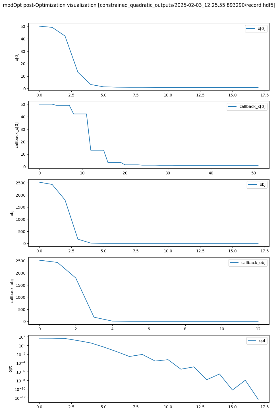
The following code plots the iterations of x[0], the objective, the Jacobian, optimality, and feasibility from the record and saves them to a file named ‘post_opt_viz.pdf’.
%matplotlib inline

from modopt.postprocessing import visualize
visualize(optimizer.out_dir+'/record.hdf5', ['x[0]', 'obj', 'opt', 'feas', 'jac[0,0]'], save_figname='post_opt_viz.pdf')
Restarting optimization: Hot-starts leveraging previous records
In practical situations, users may need to rerun a previously completed optimization if it terminates before reaching a sufficiently optimal solution. For instance, this may occur when an algorithm exits due to reaching the iteration limit or loosely set convergence tolerances. In such cases, the optimization must be re-executed with a higher iteration limit or tighter tolerances to achieve the desired results. When the problem functions and/or their derivatives are costly to evaluate, even a few reruns can significantly increase the overall optimization time, making it highly inefficient. The hot-starting feature in modOpt utilizes the record file from a prior optimization to efficiently reuse previously computed function and derivative values, thereby avoiding unnecessary computational costs.
One key benefit of hot-starting, as opposed to simply restarting from the previous solution, is that quasi-Newton methods maintain the same Hessian approximations from the prior run during a hot-start. In contrast, normal restarting initializes the approximate Hessian as an identity matrix, potentially increasing the number of additional iterations required for convergence, even if we start from the previous solution. Furthermore, restarting resets the Lagrange multipliers, which may also necessitate additional iterations, as the convergence of optimization variables often follows the convergence of Lagrange multipliers.
To hot-start a problem, set the hot_start_from parameter when instantiating the optimizer object.
The hot_start_from parameter specifies the record from which
the data should be reused when rerunning an optimization.
Users can also set hot_start_atol and hot_start_rtol,
which define the absolute and relative tolerances for the inputs
when reusing outputs from the hot-start record.
These tolerances are particularly useful in distributed computing environments
where computations are performed across multiple processors or GPUs,
as numerical discrepancies may arise due to variations in floating-point arithmetic and parallel execution.
Both tolerances are set to zero by default.
The following code hot-starts the same problem we solved and recorded at the beginning of this page but with a tighter tolerance.
hot_start_record = optimizer.out_dir+'/record.hdf5'
optimizer = mo.TrustConstr(problem=problem,
                           solver_options={'maxiter': 100, 'gtol': 1e-14},
                           hot_start_from= hot_start_record)
results   = optimizer.solve()
optimizer.print_results()
	Solution from Scipy trust-constr:
	----------------------------------------------------------------------------------------------------
	Problem                       : constrained_quadratic
	Solver                        : scipy-trust-constr
	Method                        : tr_interior_point
	Success                       : True
	Message                       : `gtol` termination condition is satisfied.
	Status                        : 1
	Total time                    : 0.21609711647033691
	Objective                     : 1.0000064010669836
	Gradient norm                 : 2.00000640105674
	Optimality                    : 3.5429931286978106e-15
	Max. constr. violation        : 1.7763568394002505e-15
	Trust region radius           : 3197678.6801213976
	Constraint penalty            : 1.0
	Barrier parameter             : 6.400000000000003e-06
	Barrier tolerance             : 6.400000000000003e-06
	Total function evals          : 14
	Total gradient evals          : 14
	Total Hessian evals           : 0
	Total constraint evals        : 14
	Total constr. Jacobian evals  : 14
	Total constr. Hessian evals   : 0
	Total iterations              : 20
	CG iterations                 : 13
	CG stop condition             : 1
	Total callbacks               : 56
	Reused callbacks              : 52
	obj callbacks                 : 14
	grad callbacks                : 14
	hess callbacks                : 0
	con callbacks                 : 14
	jac callbacks                 : 14
	----------------------------------------------------------------------------------------------------
/Users/venv/lib/python3.9/site-packages/scipy/optimize/_differentiable_functions.py:504: UserWarning: delta_grad == 0.0. Check if the approximated function is linear. If the function is linear better results can be obtained by defining the Hessian as zero instead of using quasi-Newton approximations.
  self.H.update(delta_x, delta_g)
From the console output above, we see that out of the 56 callbacks made by the optimizer, 52 were reused from the previous record and were never recomputed using the user-provided functions. Only one new evaluation of the objective, gradient, constraint, and Jacobian was performed to achieve a more optimal solution necessitated by the tighter tolerance.
For more details on any of the post-processing utilities, visit the API Reference page.